Contents
You read The cat ran away because it was scared and know at once who was scared. A language model never sees those words. It receives a list of integers, turns them into rows of decimals, and does arithmetic on the rows until a probability comes out.
This post follows that one sentence through GPT-2 small, from the first integer to the next word. If you came from our Reel, this is the long version, and it goes further in one place: it checks what the Reel's most striking number really means. Every number about the model comes from its real weights, and the code at the end reproduces the main ones.
From Text to Integers #
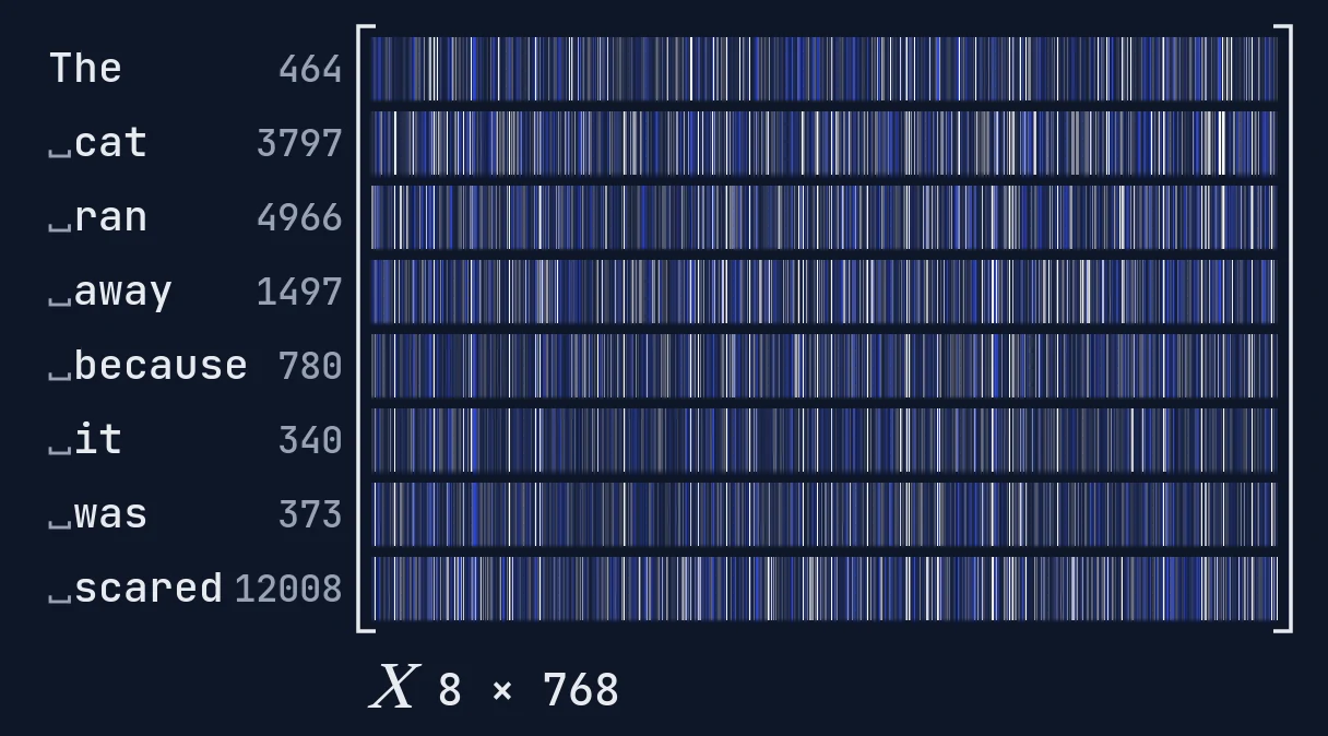
A tokenizer cuts the text into pieces from a fixed vocabulary and replaces each piece with its position in that vocabulary. Our sentence becomes eight integers:
| Token | ID |
|---|---|
"The" |
464 |
" cat" |
3797 |
" ran" |
4966 |
" away" |
1497 |
" because" |
780 |
" it" |
340 |
" was" |
373 |
" scared" |
12008 |
The space belongs to the word after it, so " cat" is not "cat". They are different tokens with different IDs, 3797 and 9246, and so are " Cat" (5181) and " CAT" (38348). Until training says otherwise, these are unrelated integers.
Tokens are not words either. GPT-2 uses byte pair encoding, which starts from single bytes and keeps merging the most frequent adjacent pair.[1] Its vocabulary is 256 bytes, 50,000 merges and one end-of-text marker, 50,257 tokens in all. Common words survive in one piece and rare ones break: " unbelievable" is one token, " tokenization" is two (" token", "ization"), and "Deeptext" is four ("D", "ee", "pt", "ext").
From Integers to Vectors #
An ID is an index into a matrix with one row per token, the embedding table E \in \mathbb{R}^{50257 \times 768}. If e_t is the one-hot vector for token t, the lookup is a multiplication:
The table holds 38,597,376 numbers, 31% of GPT-2's 124,439,808 parameters.
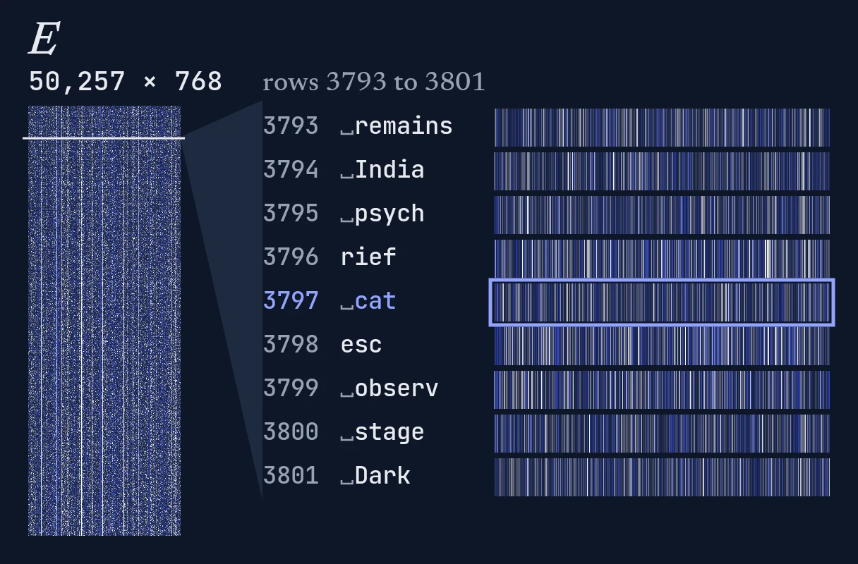
Nobody chose these values. The rows start random, and training nudges them together with the rest of the model so that the next token becomes more likely. No column means animal or plural. Whatever meaning the rows hold, it lives in how they relate to each other.
A lookup knows nothing about order, so GPT-2 keeps a second table P \in \mathbb{R}^{1024 \times 768} with one row per position, and adds it.[2] That table is also why the model reads at most 1,024 tokens at a time. Token i of the sentence, with ID t_i, becomes
Stack the eight rows and the sentence is a matrix X \in \mathbb{R}^{8 \times 768}.
Comparing Two Vectors #
Almost everything from here on is one operation. The dot product multiplies two vectors component by component and adds the results:
These are the first components of the rows for " cat" and " dog", and the first terms of their dot product:
Each term is tiny. The largest of the 768 is 0.140, and 68% of them are positive, so the total of 5.756 is the result of many small agreements. No single component decides.
- cat and dog
- cat and car
A long vector scores high against everything, so we divide by the two lengths. What remains is the cosine of the angle between the vectors, a number between -1 and 1:
Here is " cat" against other rows of the table. The last column repeats the comparison after subtracting the mean of all rows.
| Word | Cosine with " cat" |
After subtracting the mean |
|---|---|---|
" cats" |
0.693 | 0.623 |
" dog" |
0.550 | 0.489 |
" kitten" |
0.501 | 0.357 |
" rabbit" |
0.436 | 0.313 |
" car" |
0.381 | 0.329 |
" horse" |
0.362 | 0.252 |
" truck" |
0.269 | 0.140 |
" bank" |
0.239 | 0.147 |
" table" |
0.210 | 0.123 |
" idea" |
0.201 | 0.092 |
Two things stand out. The first is that nothing is near zero. The average cosine between " cat" and all 50,257 rows is 0.205, and 98% of them fall between 0.118 and 0.303. All rows share a common direction, so in this table 0.20 means unrelated. Subtract the mean row and that average drops to 0.003, which is why the last column is the fairer ruler.
The second is " car". It scores below " dog", but 0.381 is higher than 99.93% of the vocabulary. A car is not an animal, yet both are common concrete nouns that fill similar places in sentences, and those places are what the table learns.[3] What it cannot see is spelling. " cat" and " car" differ by one letter, but the model only ever receives 3797 and 1097.
Why a Word Needs Its Neighbours #
The row for " it" is the same in every sentence GPT-2 will ever read, so on its own it cannot say what it refers to. Attention is how the other tokens get in.
The model is a stack of 12 layers, and each layer runs 12 attention heads side by side. We will follow one of them: layer 4, head 3, counting from 0. Its input has the same shape as before, X \in \mathbb{R}^{8 \times 768}, but it is no longer the embedding. The sentence has already passed through four layers, and then through layer normalization.[4]
The head multiplies X by three learned matrices, which gives every token three shorter vectors:
It helps to read row q_i as what token i is looking for, k_j as what token j offers, and v_j as what token j hands over if it is chosen.[5] That is a picture and not a rule: to the model they are three linear maps. In the code they come from one matrix of shape 768 × 2304 called c_attn, cut into three parts, and then into 12 heads of 64 numbers each.
Scores #
How well a query matches a key is a dot product again. For all pairs at once:
Here d_k = 64. For the query of " it" and the key of " cat", that is 6.34 / \sqrt{ 64 } = 0.79. This is the whole grid, with queries as rows and keys as columns:
Why divide by \sqrt{d_k}? If the components of q and k are independent, with mean 0 and variance 1, their dot product has mean 0 and variance d_k, so its typical size grows like \sqrt{d_k}.[5:1]
- \sqrt{d}
- Measured on random vectors
Large scores push the next step against its ceiling, where one token takes everything and the gradients nearly vanish. For " it", the undivided dot products run from −30.3 to 6.3. Softmax, which comes next, would give " cat" a weight of 1.0000 and the runner-up about 3 \times 10^{-10}. The model was trained with the division, so this only shows the scale of the problem, but the division is the reason the real weight is 0.876 and not 1.
The Mask #
GPT-2 is trained to predict the next token, so a token must not see what comes after it. Before the next step, every score above the diagonal is replaced with -\infty, which guarantees a weight of exactly 0. This one rule matters more than it looks, and we will come back to it.
Softmax #
Softmax turns each row of scores into weights that are positive and add up to 1:
For the row of " it":
| Token | Score | exp(score) | Weight |
|---|---|---|---|
"The" |
−1.97 | 0.140 | 0.055 |
" cat" |
0.79 | 2.210 | 0.876 |
" ran" |
−3.02 | 0.049 | 0.019 |
" away" |
−2.57 | 0.077 | 0.030 |
" because" |
−3.79 | 0.023 | 0.009 |
" it" |
−3.70 | 0.025 | 0.010 |
| Sum | 2.523 | 1.000 |
The exponential rewards gaps. " cat" leads "The" by 2.76 in score, and that becomes a factor of 15.8 in weight. Here are all the rows, with the masked cells left empty:
The Output #
The output for each token is the weighted sum of the value vectors:
For " it", that is
Almost all of it comes from " cat". The cosine between z_{\text{it}} and v_{\text{cat}} is 0.999. This is the number behind the closing line of the Reel, and it is tempting to stop here.
What This Head Actually Learned #
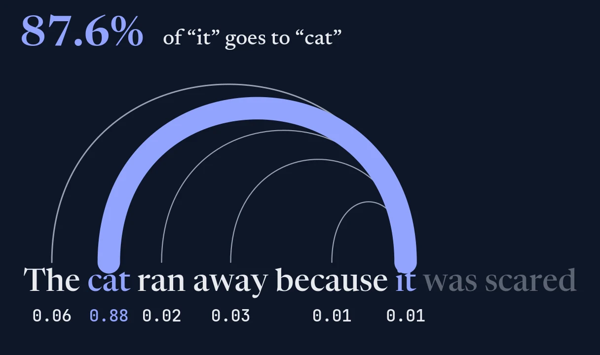
It would be easy to conclude that the model worked out what it refers to. The numbers do not support that, for three reasons.
We picked the best head. Of 144 heads, this is the only one that gives " cat" a majority. Just five rank it first, and the average weight it receives is 5.4%. The most common first choice for " it" is "The", in 113 heads.
The head does not read the sentence. Look at the grid again: every token after " cat" gives it the largest share, and " ran" gives it even more than " it" does. Change the noun, and the head follows the new noun, whether or not the sentence makes sense:
| Sentence | Largest weights of " it" |
|---|---|
| The dog ran away because it was scared | " dog" 0.86, "The" 0.06 |
| The car ran away because it was scared | " car" 0.81, "The" 0.10 |
| The animal did not cross the street because it was tired | " animal" 0.87, "The" 0.07 |
| The animal did not cross the street because it was wide | " animal" 0.87, "The" 0.07 |
| The cat chased the dog because it was angry | " dog" 0.54, " cat" 0.37 |
| The dog chased the cat because it was angry | " cat" 0.67, " dog" 0.25 |
| The trophy did not fit in the suitcase because it was too big | "The" 0.37, " suitcase" 0.28, " trophy" 0.24 |
| The trophy did not fit in the suitcase because it was too small | "The" 0.37, " suitcase" 0.28, " trophy" 0.24 |
The pairs show the real limit. Each pair differs only in the words after " it", and the weights are identical, because the mask hides those words. So " scared" played no part in the 87.6%. With two nouns the head hedges, and the trophy pair, a classic Winograd schema,[6] leaves it undecided. What it has learned is narrower than reference: look back for a likely noun. That is a useful feature, and in our sentence it happens to land on the right word. Later tokens can still do better, because " scared" can see everything before it.
One head barely moves the vector. z_{\text{it}} is 64 of 768 numbers, from one head of 12. Those outputs are joined, mixed and added to the token's vector, and in layer 4 the part that gets added is about a fifth as long as the vector it joins. The cosine between the vectors of " it" and " cat" is 0.636 before the layer and 0.627 after it. So nearly all cat is true of z_{\text{it}} and false of the token. Across the whole model, " it" never becomes special to " cat":
- was
- because
- cat
- The
Attention weights tell you where a number came from. They do not tell you why the model behaves as it does.[7]
One Head Is Not the Model #
Say h is a token's vector as it enters a layer. The 12 outputs of 64 numbers are joined back into 768, multiplied by one more matrix and added to h. A small network then widens the result to 3,072 numbers, applies GELU, narrows it back to 768, and adds that too:
The additions are residual connections,[8] and they are why a layer adjusts a vector instead of replacing it. Each of these layers has 7,087,872 parameters, and there are 12 of them, which gives 144 heads doing different things.
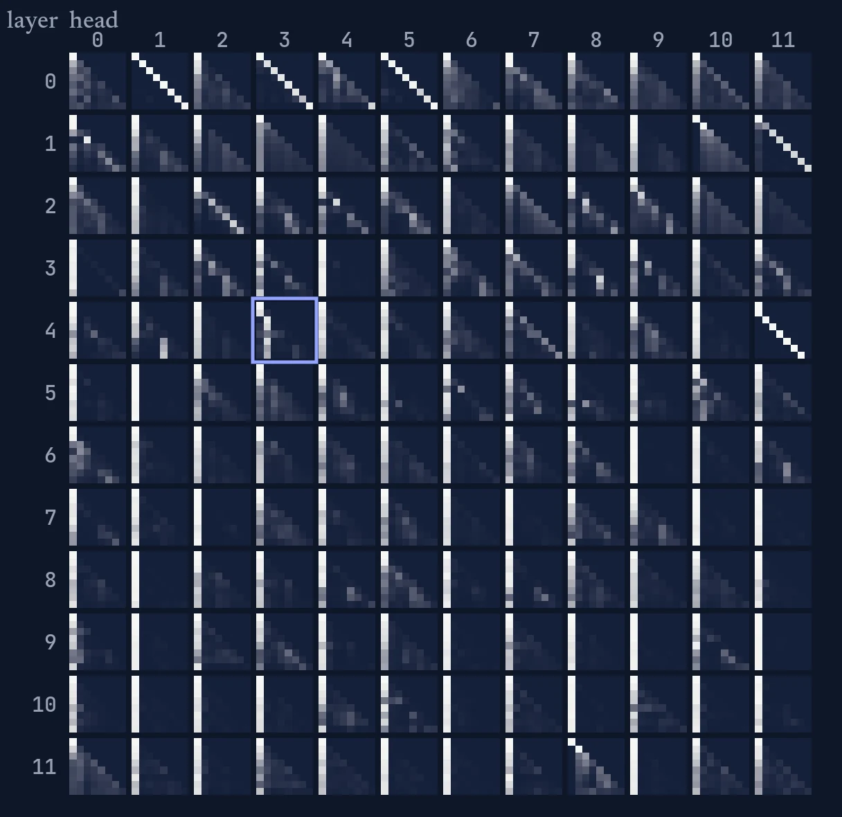
Larger models repeat the same block with more of everything. All four versions of GPT-2 share the vocabulary and the limit of 1,024 tokens:
| Model | Layers | Heads | Vector size |
|---|---|---|---|
| GPT-2 small | 12 | 12 | 768 |
| GPT-2 medium | 24 | 16 | 1,024 |
| GPT-2 large | 36 | 20 | 1,280 |
| GPT-2 XL | 48 | 25 | 1,600 |
Back to Words #
After the last layer and one more normalization, the vector of the last token is multiplied by E. It is the same matrix as at the start: GPT-2 reuses its embedding table as its output layer, which is called weight tying.[9]
That is a dot product with each of the 50,257 rows, the same operation for the third time. A token scores high when its row lines up with the model's final vector, and softmax turns the scores into probabilities. After The cat ran away because it was scared, the top five are:
| Next token | ID | Probability |
|---|---|---|
" of" |
286 | 25.2% |
"." |
13 | 21.8% |
"," |
11 | 11.5% |
" and" |
290 | 10.3% |
","" |
553 | 4.6% |
These five hold 73.4% of the probability, and the top 20 hold 90.7%. The winner has only 25.2%, so the model is far from sure. Always taking the top token is called greedy decoding, and most applications sample from p instead. Either way, one new ID joins the list, here 286 for " of", and everything runs again.
In Code #
This loads GPT-2 small and reproduces the main numbers of the post, computing the head by hand from its own weights.
import torch
from transformers import GPT2LMHeadModel, GPT2TokenizerFast

name = "gpt2"
tokenizer = GPT2TokenizerFast.from_pretrained(name)
model = GPT2LMHeadModel.from_pretrained(name, attn_implementation="eager")
model.eval()

text = "The cat ran away because it was scared"
ids = tokenizer(text, return_tensors="pt").input_ids
print(ids[0].tolist())
# [464, 3797, 4966, 1497, 780, 340, 373, 12008]

# Cosines between rows of the embedding table
E = model.transformer.wte.weight.detach()
cosine = torch.nn.functional.cosine_similarity
print(f"{cosine(E[3797], E[3290], dim=0):.3f}")  # cat, dog
# 0.550
print(f"{cosine(E[3797], E[1097], dim=0):.3f}")  # cat, car
# 0.381

with torch.no_grad():
    output = model(ids, output_attentions=True, output_hidden_states=True)

    # Layer 4, head 3, by hand. hidden_states[4] enters layer 4.
    block = model.transformer.h[4]
    X = block.ln_1(output.hidden_states[4][0])
    Q, K, V = block.attn.c_attn(X).split(768, dim=-1)
    Q, K, V = (m[:, 3 * 64 : 4 * 64] for m in (Q, K, V))

    S = Q @ K.T / 64**0.5
    mask = torch.tril(torch.ones(8, 8, dtype=torch.bool))
    a = S.masked_fill(~mask, float("-inf")).softmax(dim=-1)
    z = a @ V

print(f"{a[5, 1]:.3f}")  # " it" to " cat"
# 0.876
print(f"{cosine(z[5], V[1], dim=0):.3f}")  # z_it, v_cat
# 0.999

# The same weights, as the model reports them
print(torch.allclose(a, output.attentions[4][0, 3], atol=1e-5))
# True

# The next token
top = output.logits[0, -1].softmax(dim=-1).topk(5)
for p, i in zip(top.values, top.indices):
    print(f"{tokenizer.decode(i)!r:7} {p:.3f}")

# ' of'   0.252
# '.'     0.218
# ','     0.115
# ' and'  0.103
# ',"'    0.046
Common Mistakes #
- Counting words when the model counts tokens. Limits and prices are in tokens, and a rare word can cost several.
- Reading a meaning into one column of an embedding. Columns have no names, and nothing in the model says what any of them should mean.
- Treating a cosine of 0 as the mark of unrelated words. In GPT-2's table, that mark is about 0.2.
- Reading an attention map as an explanation. One head on one sentence shows what happened there, so try other sentences and other heads before concluding anything.
- Forgetting that the mask works per position. A token cannot use what comes after it, but the tokens after it can use it.
- Thinking of queries, keys and values as a database lookup. Nothing is retrieved exactly: every value goes into the sum, in some proportion.
R. Sennrich, B. Haddow and A. Birch, Neural machine translation of rare words with subword units, ACL 2016. ↩︎
A. Radford et al., Language models are unsupervised multitask learners, OpenAI, 2019. ↩︎
J. R. Firth, A synopsis of linguistic theory 1930–1955, 1957. The idea that a word is known by the company it keeps. ↩︎
J. Ba, J. Kiros and G. Hinton, Layer normalization, 2016. ↩︎
A. Vaswani et al., Attention is all you need, NeurIPS 2017. ↩︎ ↩︎
H. Levesque, E. Davis and L. Morgenstern, The Winograd schema challenge, KR 2012. ↩︎
S. Jain and B. Wallace, Attention is not explanation, NAACL 2019. ↩︎
K. He, X. Zhang, S. Ren and J. Sun, Deep residual learning for image recognition, CVPR 2016. ↩︎
O. Press and L. Wolf, Using the output embedding to improve language models, EACL 2017. ↩︎
Comments
Loading comments…